Divide and conquer

A divide and conquer algorithm is a strategy of solving a large problem by

breaking the problem into smaller sub-problems

solving the sub-problems, and

combining them to get the desired output.

To use the divide and conquer algorithm, recursion is used.

How Divide and Conquer Algorithms Work?

Here are the steps involved:

Divide: Divide the given problem into sub-problems using recursion.

Conquer: Solve the smaller sub-problems recursively. If the subproblem is small enough, then solve it directly.

Combine: Combine the solutions of the sub-problems that are part of the recursive process to solve the actual problem.

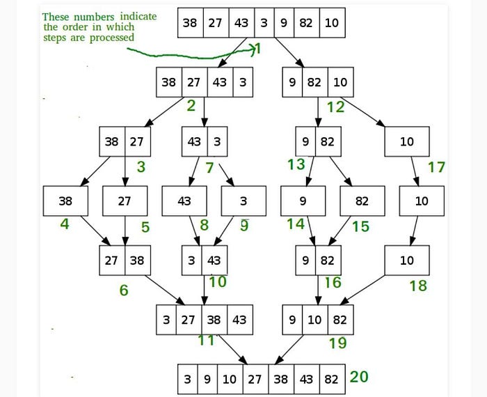
Let the given array be:

initial array for merge sort

Array for merge sort

Divide the array into two halves.

Divide the array into two subparts

Divide the array into two subparts

Again, divide each subpart recursively into two halves until you get individual elements.

Divide the array into smaller subparts

Divide the array into smaller subparts

Now, combine the individual elements in a sorted manner. Here, conquer and combine steps go side by side.

Combine the subparts

Combine the subparts

Time Complexity

The complexity of the divide and conquer algorithm is calculated using the master theorem.

T(n) = aT(n/b) + f(n),

where,

n = size of input

a = number of subproblems in the recursion

n/b = size of each subproblem. All subproblems are assumed to have the same size.

f(n) = cost of the work done outside the recursive call, which includes the cost of dividing the problem and cost of merging the solutions

Let us take an example to find the time complexity of a recursive problem.

For a merge sort, the equation can be written as:

T(n) = aT(n/b) + f(n)

= 2T(n/2) + O(n)

Where,

a = 2 (each time, a problem is divided into 2 subproblems)

n/b = n/2 (size of each sub problem is half of the input)

f(n) = time taken to divide the problem and merging the subproblems

T(n/2) = O(n log n) (To understand this, please refer to the master theorem.)

Now, T(n) = 2T(n log n) + O(n)

≈ O(n log n).

Divide and Conquer Vs Dynamic approach

The divide and conquer approach divides a problem into smaller subproblems; these subproblems are further solved recursively. The result of each subproblem is not stored for future reference, whereas, in a dynamic approach, the result of each subproblem is stored for future reference.

Use the divide and conquer approach when the same subproblem is not solved multiple times. Use the dynamic approach when the result of a subproblem is to be used multiple times in the future.

Let us understand this with an example. Suppose we are trying to find the Fibonacci series. Then,

Divide and Conquer approach:

fib(n)

If n < 2, return 1

Else , return f(n — 1) + f(n -2)

Dynamic approach:

mem = []

fib(n)

If n in mem: return mem[n]

else,

If n < 2, f = 1

else , f = f(n — 1) + f(n -2)

mem[n] = f

return f

In a dynamic approach, mem stores the result of each subproblem.

Advantages of Divide and Conquer Algorithm

The complexity for the multiplication of two matrices using the naive method is O(n3), whereas using the divide and conquer approach (i.e. Strassen’s matrix multiplication) is O(n2.8074). This approach also simplifies other problems, such as the Tower of Hanoi.

This approach is suitable for multiprocessing systems.

It makes efficient use of memory caches.

Divide and Conquer Applications

Binary Search

Merge Sort

Quick Sort

Strassen’s Matrix multiplication

Karatsuba Algorithm.

A classic example of Divide and Conquer is Merge Sort demonstrated below. In Merge Sort, we divide array into two halves, sort the two halves recursively, and then merge the sorted halves.

def bsearch(list, val):

list_size = len(list) — 1

idx0 = 0

idxn = list_size

# Find the middle most value

while idx0 <= idxn:

midval = (idx0 + idxn)// 2

if list[midval] == val:

return midval

# Compare the value the middle most value

if val > list[midval]:

idx0 = midval + 1

else:

idxn = midval — 1

if idx0 > idxn:

return None

# Initialize the sorted list

list = [2,7,19,34,53,72]

# Print the search result

print(bsearch(list,72))

print(bsearch(list,11))

When the above code is executed, it produces the following result:

5

None